In the previous article we wrote a Python function which utilised the Polygon API to extract a month of minutely data for both a major (EURUSD) and exotic (MZXZAR) FX pair. We plotted the returns series and looked at some of the issues that can occur when working with this type of data. This article is part of series where we will be creating a machine learning model which uses realised volatility to predict market regime change. In this article we will be learning how to calculate realised volatility. We will also be conducting a exploratory data analysis to prepare the feature set for our machine learning model.

In order to follow along with the code in this tutorial you will need:

• Python 3.9
• Matplotlib 3.5
• Pandas 1.4
• Requests 2.27
• Seaborn 0.12.

We also recommend that you take a look at our early career research series to create an algorithmic trading environment inside a Jupyter Notebook.

Realised Volatility

In order to calculate realised volatility we first need to obtain and format the data. In the previous article we created Python functions to contact the Polygon API and obtain a month of minutely data for EURUSD and MZXZAR. You can view the full article here. Below you will find the code to obtain the data.

import json
import matplotlib.pyplot as plt
import pandas as pd
import requests
import seaborn as sns


POLYGON_API_KEY = os.getenv("POLYGON_API_KEY")
HEADERS = {
    'Authorization': 'Bearer ' + POLYGON_API_KEY
}
BASE_URL = 'https://api.polygon.io/v2/aggs/'


def get_fx_pairs_data(pg_tickers):
    start = '2023-01-01'
    end = '2023-01-31'
    multiplier = '1'
    timespan = 'minute'
    fx_url = f"range/{multiplier}/{timespan}/{start}/{end}?adjusted=true&sort=asc&limit=50000"
    fx_pairs_dict = {}
    for pair in pg_tickers:
        response = requests.get(
            f"{BASE_URL}ticker/{pair}/{fx_url}", 
            headers=HEADERS
        ).json()
        fx_pairs_dict[pair] = pd.DataFrame(response['results'])
    return fx_pairs_dict


def format_fx_pairs(fx_pair_dict):
    for pair in fx_pairs_dict.keys():
        fx_pairs_dict[pair]['t'] = pd.to_datetime(fx_pairs_dict[pair]['t'],unit='ms')
        fx_pairs_dict[pair] = fx_pairs_dict[pair].set_index('t')
    return fx_pairs_dict


def create_str_index(fx_pairs_dict):
    fx_pairs_str_ind = {}
    for pair in fx_pairs_dict.keys():
        fx_pairs_str_ind[pair] = fx_pairs_dict[pair].set_index(
            fx_pairs_dict[pair].index.to_series().dt.strftime(
                '%Y-%m-%d-%H-%M-%S'
            )
        )
    return fx_pairs_str_ind


def create_returns_series(fx_pairs_str_ind):
    for pair in fx_pairs_str_ind.keys():
    fx_pairs_str_ind[pair]['rets'] = fx_pairs_str_ind[pair]['c'].pct_change()
    return fx_pair_str_ind 

The functions can be called in a new cell or in a main if running the code outside a notebook environment. The code below will store the returns value of each function in a variable.

pg_tickers = ["C:EURUSD", "C:MXNZAR"]
fx_pairs_dict = get_fx_pairs_data(pg_tickers)
formatted_fx_dict = format_fx_pairs(fx_pairs_dict)
fx_pairs_str_ind = create_str_index(formatted_fx_dict)
fx_returns_dict = create_returns_series(fx_pairs_str_ind) 

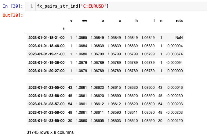
The FX data for each pair can be accessed as below:

fx_returns_dict['C:EURUSD']

Realized volatility is a measure of risk. It measures the variability in an investment over a defined period of time. It is calculated as the square root of the sum of the squared return for a particular period of time. In contrast to implied volatility, realised volatility shows the actual change in historical prices, rather than a prediction of future volatility. However, it is possible to use the data to forecast the volatility in returns.

So why is this useful? If you can reliably predict volatility for a window of future time you can make an assessment of the market regime. This can help you determine the types of trading strategies you may want to use. For example in periods of low volatility you might look at trend following strategies on stocks. In a high volatility environment you might want to consider mean reverting strategies or options trading strategies such as Straddle or Strangle. By quantifying the level of risk present in your trading universe you can make better trading decisions.

Realised volatility is a way of understanding the degree of price movement for a given period. It is calculated as follows:

1. Collect the price data and calculate the returns
2. Square the returns to give more weight to larger changes
3. Calculate the average of the squared returns by adding them up and dividing by the number of periods (this is also known as the variance)
4. Take the square root of the variance (also know as the standard deviation). This is your measure of realised volatility

Ultimately we will be training a Support Vector Regressor to help us identify market regime change. In order to do this we will calculate realised volatility across a particular window of time. The window you select will depend upon the frequency of you data and the liquidity of the asset. As we are considering both a major and minor FX pair we will calculate our realised volatility over 30 data points. The Pandas library contains a rolling function that can be applied to any statistical aggregator using method chaining. Here we use rolling() with std(), to calculate rolling standard deviation. The rolling window size can be set to any number of fixed observations or timedeltas, such as business days.

Calculating Realised Volatility

The code below will create a new column in each of the fx pairs DataFrames which will contain the realised vol calculated as the rolling standard deviation of the last 30 data points. This will equate approximately to the last 30 minutes of data, with some variation depending on the trading frequency of the FX pair. Let's take a look at the realised volatility on a chart.

def create_realised_vol:
for pair in pairs_rets_dict:
    pairs_rets_dict[pair]['realised_vol'] = pairs_rets_dict[pair]['rets'].rolling(30).std()
return pairs_rets_dict 

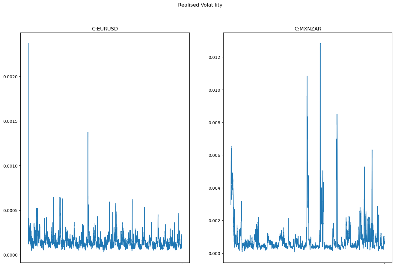
As you can see the exotic pair MXNZAR has fewer data points than EURUSD, as it is thinly traded this is to be expected. In fact if we look at the length of both our DataFrames we can see that EURUSD has 31745 rows, whereas MXNZAR has 16865 rows almost half as many. In the previous article we discussed different options available to us that would allow us to handle the missing data points in the MXNZAR pair.

Exploring the Features of the Data

Before we begin to construct a machine learning model it is a good idea to have a look at the data and understand how its features could affect model performance. Why should you do this, why can't you just get going? Well, firstly the distribution of the data should influence your choice of model. For example, if your data was linearly distributed the use of linear regression model or a linear kernel in an SVM would be appropriate. If the data is non-lineaer a polynomial regression or radial basis function kernel would be more appropriate. You might also want to consider transforming or scaling your data to make it more compatible with your chosen model. Perharps your data contains outliers or missing data that you need to be aware of. There could be correlation (or linear association) between the features you have selected to train your model. There are many reasons why it is important to get to know your data before you start training a model. In fact it's estimated that between 70-80% of an engineer's time if spend toiling with data. Let's take a look at a simple exploratory data analysis:

First we will look at the distribution of the returns for both our FX pairs. We use the Seaborn function kdeplot() to visualise the distributions.

fig, ax = plt.subplots(2,2, figsize=(16, 10), squeeze=False)
y_data = ['rets', 'realised_vol']
for idx, fxpair in enumerate(fx_pairs_str_ind.keys()):
    for idx2, dfcol in enumerate(y_data):
        row = (idx)
        col = (idx2%2)
        sns.kdeplot(fx_pairs_str_ind[fxpair][dfcol], ax=ax[row][col], bw_adjust=0.5)
        ax[row][col].set_title(fxpair)
fig.suptitle("KDE of Returns & Realised Volatility")
plt.show() 

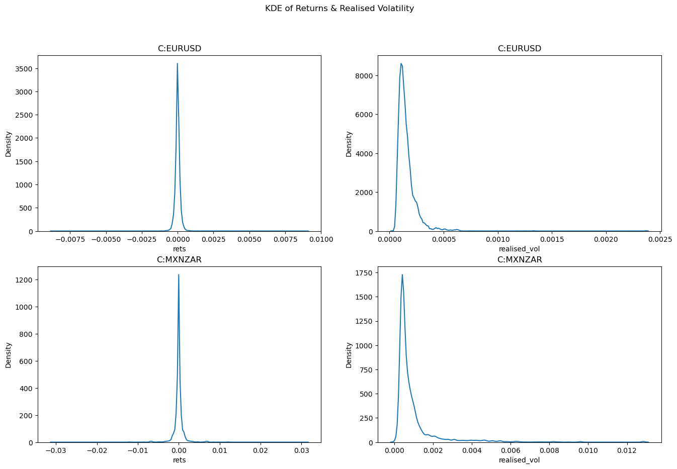
Firstly it's important to note that the scale on the x axis for EURUSD and MXNZAR is different. The range of returns is larger for MXNZAR in both the poistive and negative direction when compare to EURUSD. This is reflected in the realised volatility. We can also see that we have positive kurtosis of all distributions when compared to a standard normal distribution. The realised volatility also have positive skew. This information will be helpful when we are trying to choose or improve any machine learning models that we might want to use. Finally in the exoctic FX pair MXNZAR, we can see two small humps just before -0.01 and 0.01. This indicates the presence of spikes in our returns data.

To look into these with more detail we can use Violin plot. This will allows us to see how many instances of these spikes there are in our data and how far from the bulk of the distribution they are. The following code will create the violin plot.

fig, ax = plt.subplots(1,2, figsize=(16, 10), squeeze=False)

for idx, fxpair in enumerate(fx_pairs_str_ind.keys()):
    row = (idx//2)
    col = (idx%2)
    sns.violinplot(x='rets', data=fx_pairs_str_ind[fxpair], ax=ax[row][col], inner='point')
    ax[row][col].set_title(fxpair)
fig.suptitle("Violin plot of rets")
plt.show() 

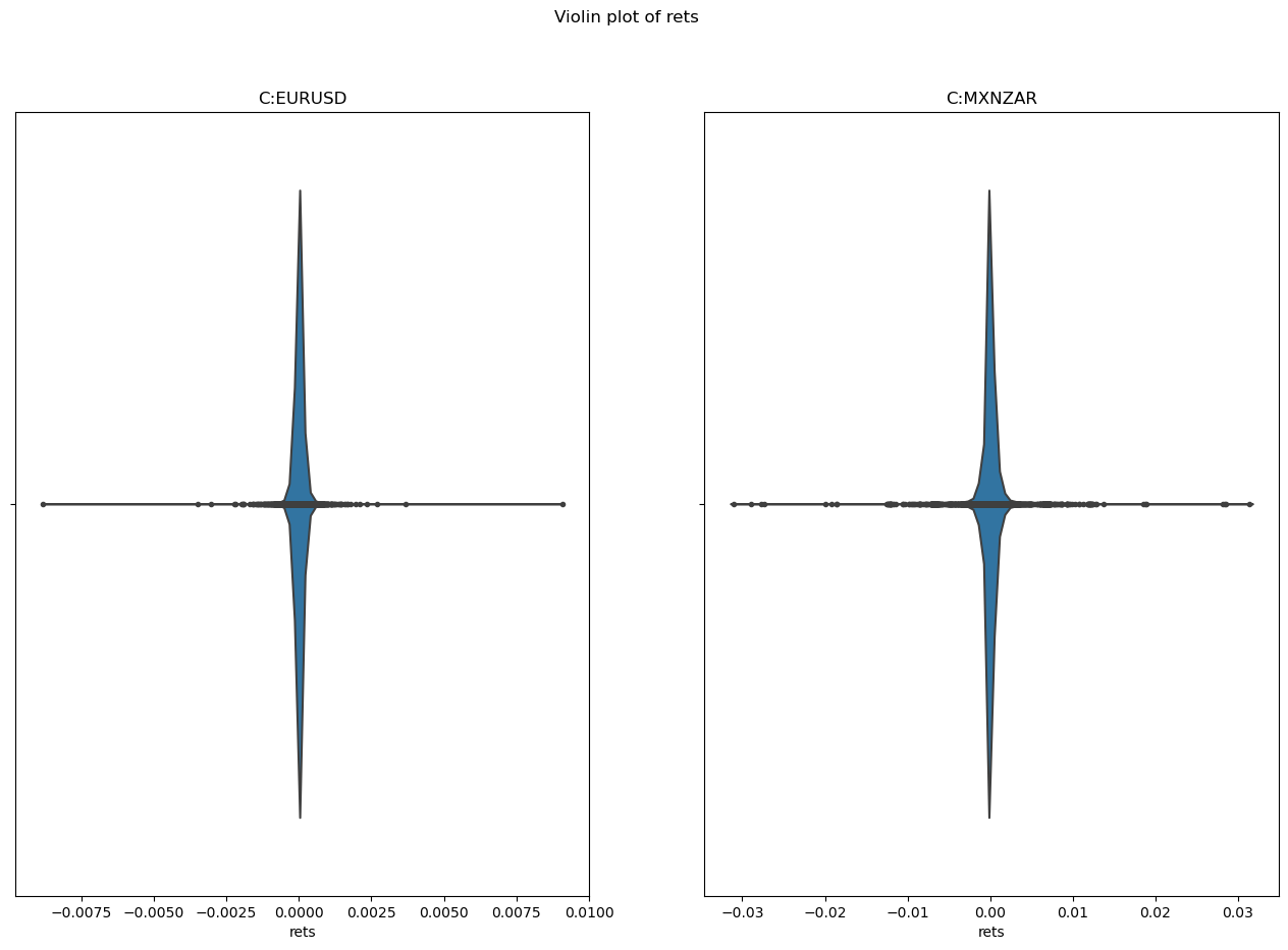
As you can see there are more points further from the bulk of the distribution in the MXNZAR FX pair. This means that there are more occassions where there is a higher or lower return when compared to the EURUSD. This information alone could be useful when you are considering trading strategies.

As we are planning to put our data into a machine learning model we also need to think about correlation. We want to use the realised volatility and the returns as features in a training set for a Support Vector Regressor. We need to ensure that these two features aren't correlated, otherwise we would be giving the machine learning model the same information twice. The model would become overspecified which could lead to poor model performance. Below we will look at the correlation between our two chosen features. In order to use both features we would be looking for a correlation close to zero.

The following function will display a scatter plot of the two columns; returns and realised vol. It also uses the Pandas pd.DataFrame.corr method to calculate the correlation between the two.

fig, ax = plt.subplots(1,2, figsize=(16, 10), squeeze=False)
for idx, fxpair in enumerate(fx_pairs_str_ind.keys()):
    row = (idx//2)
    col = (idx%2)
    print(f"vol and rets correlation for {fxpair} is " 
        f"{fx_pairs_str_ind[fxpair]['rets'].corr(fx_pairs_str_ind[fxpair]['realised_vol'])}")
    sns.scatterplot(data=fx_pairs_str_ind[fxpair], x='rets', y='realised_vol', ax=ax[row][col])
    ax[row][col].set_title(fxpair)
fig.suptitle("Correlation between realised vol and returns")
plt.show()

vol and rets correlation for C:EURUSD is 0.008572524273933109
vol and rets correlation for C:MXNZAR is 0.018750753882674935 

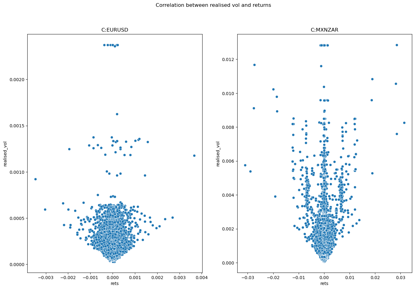
Now that we know our returns series and realised vol have little correlation we can use them as separate features in our machine learning model. In the next article we will be building a Support Vector Regressor to determine how reliably we can predict the next value of realised volatility using the returns and realised volatility values from the previous time point. This will allow us to prepare a pipeline for our data, understand some of the model parameters and prepare for the final specification of the model.

Related Articles

• Creating a Returns Series with Polygon's Forex Data